gftool.fourier.tau2iw_ft_lin

gftool.fourier.tau2iw_ft_lin(gf_tau, beta)

Fourier integration of the real Green’s function gf_tau.

Fourier transformation of a fermionic imaginary-time Green’s function to Matsubara domain. We assume a real Green’s function gf_tau, which is the case for commutator Green’s functions \(G_{AB}(τ) = ⟨A(τ)B⟩\) with \(A = B^†\). The Fourier transform gf_iw is then Hermitian. Filon’s method is used to calculated the Fourier integral

\[G^n = 0.5 ∫_{-β}^{β}dτ G(τ) e^{iω_n τ},\]

\(G(τ)\) is approximated by a linear spline. A linear approximation was chosen to be able to integrate noisy functions. Information on oscillatory integrations can be found e.g. in [filon1930] and [iserles2006].

Parameters

gf_tau(…, N_tau) float np.ndarray

The Green’s function at imaginary times \(τ \in [0, β]\).

betafloat

The inverse temperature \(beta = 1/k_B T\).

Returns

gf_iw(…, (N_iw - 1)/2) float np.ndarray

The Fourier transform of gf_tau for positive fermionic Matsubara frequencies \(iω_n\).

See also

tau2iw_dft

Plain implementation using Riemann sum.

References

filon1930

Filon, L. N. G. III.—On a Quadrature Formula for Trigonometric Integrals. Proc. Roy. Soc. Edinburgh 49, 38–47 (1930). https://doi.org/10.1017/S0370164600026262

iserles2006

Iserles, A., Nørsett, S. P. & Olver, S. Highly Oscillatory Quadrature: The Story so Far. in Numerical Mathematics and Advanced Applications (eds. de Castro, A. B., Gómez, D., Quintela, P. & Salgado, P.) 97–118 (Springer, 2006). https://doi.org/10.1007/978-3-540-34288-5_6 http://www.sam.math.ethz.ch/~hiptmair/Seminars/OSCINT/INO06.pdf

Examples

>>> BETA = 50
>>> tau = np.linspace(0, BETA, num=2049, endpoint=True)
>>> iws = gt.matsubara_frequencies(range((tau.size-1)//2), beta=BETA)

>>> poles = 2*np.random.random(10) - 1  # partially filled
>>> weights = np.random.random(10)
>>> weights = weights/np.sum(weights)
>>> gf_tau = gt.pole_gf_tau(tau, poles=poles, weights=weights, beta=BETA)
>>> # 1/z tail has to be handled manually
>>> gf_ft_lin = gt.fourier.tau2iw_ft_lin(gf_tau + .5, beta=BETA) + 1/iws
>>> gf_tau.size, gf_ft_lin.size
(2049, 1024)
>>> gf_iw = gt.pole_gf_z(iws, poles=poles, weights=weights)

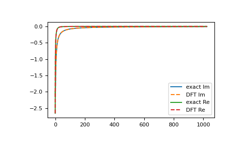
>>> import matplotlib.pyplot as plt
>>> __ = plt.plot(gf_iw.imag, label='exact Im')
>>> __ = plt.plot(gf_ft_lin.imag, '--', label='DFT Im')
>>> __ = plt.plot(gf_iw.real, label='exact Re')
>>> __ = plt.plot(gf_ft_lin.real, '--', label='DFT Re')
>>> __ = plt.legend()
>>> plt.show()

(png, pdf)

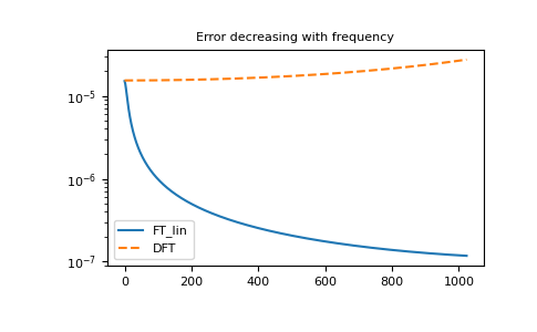
>>> __ = plt.title('Error decreasing with frequency')
>>> __ = plt.plot(abs(gf_iw - gf_ft_lin), label='FT_lin')
>>> gf_dft = gt.fourier.tau2iw_dft(gf_tau + .5, beta=BETA) + 1/iws
>>> __ = plt.plot(abs(gf_iw - gf_dft), '--', label='DFT')
>>> __ = plt.legend()
>>> plt.yscale('log')
>>> plt.show()

(png, pdf)

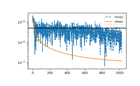
The method is resistant against noise:

>>> magnitude = 5e-6
>>> noise = np.random.normal(scale=magnitude, size=gf_tau.size)
>>> gf_ft_noisy = gt.fourier.tau2iw_ft_lin(gf_tau + noise + .5, beta=BETA) + 1/iws
>>> __ = plt.plot(abs(gf_iw - gf_ft_noisy), '--', label='noisy')
>>> __ = plt.axhline(magnitude, color='black')
>>> __ = plt.plot(abs(gf_iw - gf_ft_lin), label='clean')
>>> __ = plt.legend()
>>> plt.yscale('log')
>>> plt.show()

(png, pdf)