Tutorial

This tutorial explains some of the basic functionality. Throughout the tutorial we assume you have imported GfTool as

>>> import gftool as gt

and the packages numpy and matplotlib are imported as usual

>>> import numpy as np
>>> import matplotlib.pyplot as plt

Lattice Green’s functions

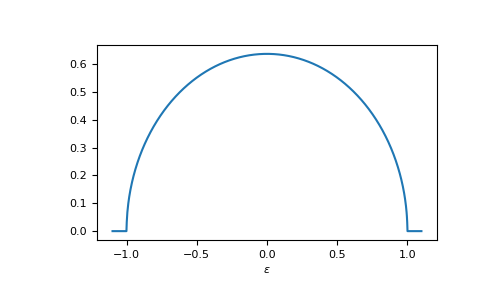
The package contains non-interacting Green’s functions for some tight-binding lattices. They can be found in gftool.lattice. E.g. the dos of the Bethe lattice, bethe:

>>> ww = np.linspace(-1.1, 1.1, num=1000)
>>> dos_ww = gt.lattice.bethe.dos(ww, half_bandwidth=1.)
>>> __ = plt.plot(ww, dos_ww)
>>> __ = plt.xlabel(r"$\epsilon$")
>>> plt.show()

(png, pdf)

Typically, a shorthand for these functions exist in the top-level module e.g. gftool.bethe_dos

>>> gt.bethe_dos is gt.lattice.bethe.dos
True

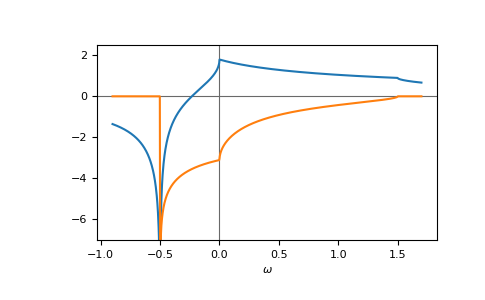
The corresponding Green’s functions are also available. The Green’s functions can be evaluate for any complex frequency, excluding the real axis, where it might become singular. E.g. the gf_z of the face-centered cubic (fcc) lattice, fcc, on a contour parallel to the real axis:

>>> ww = np.linspace(-0.9, 1.7, num=1000) + 1e-6j
>>> gf_ww = gt.lattice.fcc.gf_z(ww, half_bandwidth=1.)
>>> __ = plt.axhline(0, color="dimgray", linewidth=0.8)
>>> __ = plt.axvline(0, color="dimgray", linewidth=0.8)
>>> __ = plt.plot(ww.real, gf_ww.real)
>>> __ = plt.plot(ww.real, gf_ww.imag)
>>> __ = plt.xlabel(r"$\omega$")
>>> __ = plt.ylim(-7.0, 2.5)
>>> plt.show()

(png, pdf)

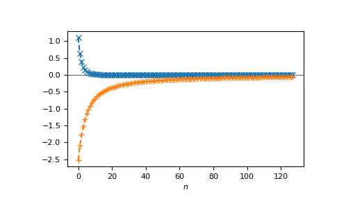
or on the Matsubara axis:

>>> beta = 50
>>> iws = gt.matsubara_frequencies(range(128), beta=beta)
>>> gf_iw = gt.lattice.fcc.gf_z(iws, half_bandwidth=1.)
>>> __ = plt.axhline(0, color="dimgray", linewidth=0.8)
>>> __ = plt.plot(gf_iw.real, "x--")
>>> __ = plt.plot(gf_iw.imag, "+--")
>>> __ = plt.xlabel("$n$")
>>> plt.show()

(png, pdf)

Density

We can also calculate the density (occupation number) from the imaginary axis for local Green’s function. We have the relation

\[⟨n⟩ = T \sum_{\{iω_n\}} \Re G(iω_n)\]

To calculate the density for a given temperature from 1024 (fermionic) Matsubara frequencies we use density_iw:

>>> temperature = 0.02
>>> iws = gt.matsubara_frequencies(range(1024), beta=1./temperature)
>>> gf_iw = gt.bethe_gf_z(iws, half_bandwidth=1.)
>>> occ = gt.density_iw(iws, gf_iw, beta=1./temperature)
>>> occ
0.5

We can also search the chemical potential \(μ\) for a given occupation using chemical_potential. To get, e.g., the Bethe lattice at quarter filling, we write:

>>> occ_quarter = 0.25
>>> def bethe_occ_diff(mu):
...     """Calculate the difference to the desired occupation, note the sign."""
...     gf_iw = gt.bethe_gf_z(iws + mu, half_bandwidth=1.)
...     return gt.density_iw(iws, gf_iw, beta=1./temperature) - occ_quarter
...
>>> mu = gt.chemical_potential(bethe_occ_diff)
>>> mu
-0.406018...

Validate the result:

>>> gf_quarter_iw = gt.bethe_gf_z(iws + mu, half_bandwidth=1.)
>>> gt.density_iw(iws, gf_quarter_iw, beta=1./temperature)
0.249999...

Fourier transform

GfTool offers also accurate Fourier transformations between Matsubara frequencies and imaginary time for local Green’s functions, see gftool.fourier. As a major part of the package, these functions are gu-functions. This is indicated in the docstrings via the shapes (…, N). The ellipsis stands for arbitrary leading dimensions. Let’s consider a simple example with magnetic splitting.

>>> beta = 20  # inverse temperature
>>> h = 0.3  # magnetic splitting
>>> eps = np.array([-0.5*h, +0.5*h])  # on-site energy
>>> iws = gt.matsubara_frequencies(range(1024), beta=beta)

We can calculate the Fourier transform using broadcasting, no need for any loops.

>>> gf_iw = gt.bethe_gf_z(iws + eps[:, np.newaxis], half_bandwidth=1)
>>> gf_iw.shape
(2, 1024)
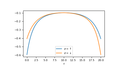
>>> gf_tau = gt.fourier.iw2tau(gf_iw, beta=beta)

The Fourier transform generates the imaginary time Green’s function on the interval \(τ ∈ [0^+, β^-]\)

>>> tau = np.linspace(0, beta, num=gf_tau.shape[-1])
>>> __ = plt.plot(tau, gf_tau[0], label=r'$\sigma=\uparrow$')
>>> __ = plt.plot(tau, gf_tau[1], label=r'$\sigma=\downarrow$')
>>> __ = plt.xlabel(r'$\tau$')
>>> __ = plt.legend()
>>> plt.show()

(png, pdf)

We see the asymmetry due to the magnetic field. Let’s check the back transformation.

>>> gf_ft = gt.fourier.tau2iw(gf_tau, beta=beta)
>>> np.allclose(gf_ft, gf_iw, atol=2e-6)
True

Up to a certain threshold the transforms agree, they are not exact inverse transformations here. Accuracy can be improved e.g. by providing (or fitting) high-frequency moments.

Single site approximation of disorder

We also offer the single site approximation for disordered Hamiltonians, namely cpa and it extension to off-diagonal disorder beb. These methods treat substitutional disorder. A multi-component system is considered, where each lattice site is randomly occupied by one of the components. The concentration of the components is known.

Coherent potential approximation (CPA)

We first consider the cpa, where only the on-site energies depend on the component. As example we consider a system of three components. We choose the on-site energies and concentrations (which should add to 1), as lattice we consider a Bethe lattice with half-bandwidth 1:

>>> from functools import partial
>>> e_onsite = np.array([-0.3, -0.1, 0.4])
>>> concentration = np.array([0.3, 0.5, 0.2])
>>> g0 = partial(gt.bethe_gf_z, half_bandwidth=1)

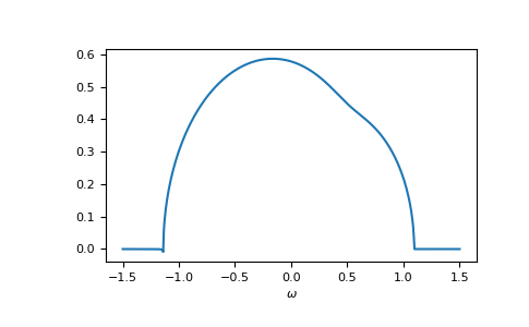
The average local Green’s function and the component Green’s functions (conditional average for local site fixed to a specific component) are calculate in CPA using an effective medium. The self-consistent effective medium is obtained via a root search using solve_root:

>>> ww = np.linspace(-1.5, 1.5, num=501) + 1e-6j
>>> self_cpa_ww = gt.cpa.solve_root(ww, e_onsite, concentration, hilbert_trafo=g0)

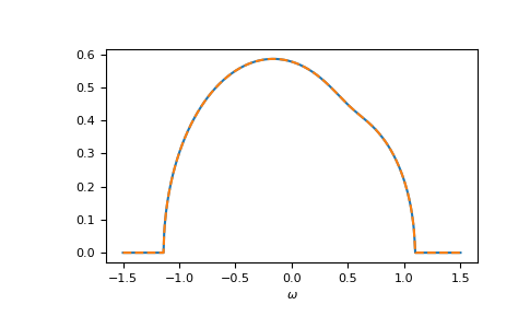
The average Green’s function is

>>> gf_coher_ww = g0(ww - self_cpa_ww)
>>> __ = plt.plot(ww.real, -1/np.pi*gf_coher_ww.imag)
>>> __ = plt.xlabel(r"$\omega$")
>>> plt.show()

(png, pdf)

For frequencies close to the real axis, issues might arise, that the conjugate solution (advanced instead of retarded) is obtained. The default restricted=True uses some heuristic to avoid this. In this example we see at the left band-edge, that for small imaginary part this can still fail. In this case, it is enough to just increase the accuracy of the root search. Additional keyword arguments are passed to scipy.optimize.root:

>>> self_cpa_ww = gt.cpa.solve_root(ww, e_onsite, concentration, hilbert_trafo=g0,
...                                 options=dict(fatol=1e-10))
>>> gf_coher_ww = g0(ww - self_cpa_ww)
>>> __ = plt.plot(ww.real, -1/np.pi*gf_coher_ww.imag)
>>> __ = plt.xlabel(r"$\omega$")
>>> plt.show()

(png, pdf)

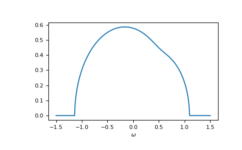
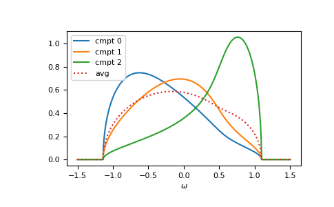
Now, everything looks fine. The component Green’s functions are calculated by gftool.cpa.gf_cmpt_z. The law of total expectation relates the component Green’s functions to the average Green’s function: np.sum(concentration*gf_cmpt_ww, axis=-1) == gf_coher_ww:

>>> gf_cmpt_ww = gt.cpa.gf_cmpt_z(ww, self_cpa_ww, e_onsite, hilbert_trafo=g0)
>>> np.allclose(np.sum(concentration*gf_cmpt_ww, axis=-1), gf_coher_ww)
True
>>> for cmpt in range(3):
...     __ = plt.plot(ww.real, -1/np.pi*gf_cmpt_ww[..., cmpt].imag, label=f"cmpt {cmpt}")
>>> __ = plt.plot(ww.real, -1/np.pi*gf_coher_ww.imag, linestyle=':', label="avg")
>>> __ = plt.legend()
>>> __ = plt.xlabel(r"$\omega$")
>>> plt.show()

(png, pdf)

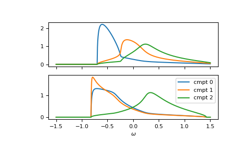
Of course, it can be calculated for any lattice Hilbert transform. Furthermore, the function is vectorized. Let’s consider a fcc lattice, where one component has different on-site energies for up and down spin. The on-site energies can simply be stacked as 2-dimensional array. We can also take the previous self-energy as a starting guess self_cpa_z0:

>>> e_onsite = np.array([[-0.3, +0.15, +0.4],
...                      [-0.3, -0.35, +0.4]])
>>> concentration = np.array([0.3, 0.5, 0.2])
>>> g0 = partial(gt.fcc_gf_z, half_bandwidth=1)
>>> self_cpa_ww = gt.cpa.solve_root(ww[:, np.newaxis], e_onsite, concentration,
...                                 hilbert_trafo=g0, options=dict(fatol=1e-8),
...                                 self_cpa_z0=self_cpa_ww[:, np.newaxis])
>>> gf_cmpt_ww = gt.cpa.gf_cmpt_z(ww[:, np.newaxis], self_cpa_ww, e_onsite, hilbert_trafo=g0)
>>> __, axes = plt.subplots(nrows=2, sharex=True)
>>> for spin, ax in enumerate(axes):
...     for cmpt in range(3):
...         __ = ax.plot(ww.real, -1/np.pi*gf_cmpt_ww[:, spin, cmpt].imag, label=f"cmpt {cmpt}")
>>> __ = plt.legend()
>>> __ = plt.xlabel(r"$\omega$")
>>> plt.show()

(png, pdf)

Blackman, Esterling, Berk (BEB)

The beb formalism is an extension of cpa to off-diagonal disorder. It allows us to provide different hopping amplitudes. We have the additional parameter hopping which gives the relative hopping amplitudes. The cpa corresponds to hopping=np.ones([N, N]), where N is the number of components. The beb module works very similar to cpa: We use solve_root to get the effective medium, in BEB, however, the effective medium is a matrix. Next the component Green’s function are calculated using gf_loc_z. These are, however, already multiplied by the concentration. So the average Green’s function is gf_loc_z.sum(axis=-1). Let’s compare cpa and beb:

>>> from functools import partial
>>> e_onsite = np.array([-0.3, -0.1, 0.4])
>>> concentration = np.array([0.3, 0.5, 0.2])
>>> hopping = np.ones([3, 3])
>>> g0 = partial(gt.bethe_gf_z, half_bandwidth=1)
>>> ww = np.linspace(-1.5, 1.5, num=501) + 1e-5j

>>> self_cpa_ww = gt.cpa.solve_root(ww, e_onsite, concentration, hilbert_trafo=g0)
>>> gf_coher_ww = g0(ww - self_cpa_ww)

>>> self_beb_ww = gt.beb.solve_root(ww, e_onsite, concentration=concentration,
...                                 hopping=hopping, hilbert_trafo=g0)
>>> gf_loc_ww = gt.beb.gf_loc_z(ww, self_beb_ww, hopping=hopping, hilbert_trafo=g0)

>>> __ = plt.plot(ww.real, -1/np.pi*gf_coher_ww.imag, label="CPA avg")
>>> __ = plt.plot(ww.real, -1/np.pi*gf_loc_ww.sum(axis=-1).imag,
...              linestyle='--', label="BEB avg")
>>> __ = plt.xlabel(r"$\omega$")
>>> plt.show()

(png, pdf)

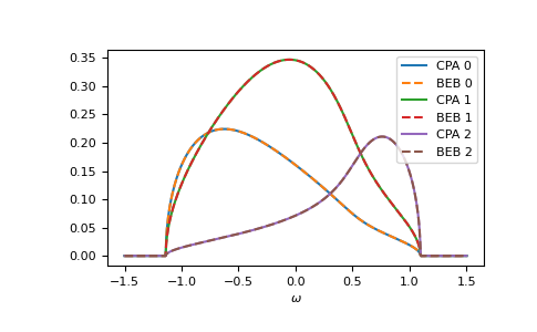
Of course, also the components match:

>>> gf_cmpt_ww = gt.cpa.gf_cmpt_z(ww, self_cpa_ww, e_onsite, hilbert_trafo=g0)
>>> c_gf_cmpt_ww = gf_cmpt_ww * concentration  # to compare with BEB
>>> for cmpt in range(3):
...     __ = plt.plot(ww.real, -1/np.pi*c_gf_cmpt_ww[..., cmpt].imag, label=f"CPA {cmpt}")
...     __ = plt.plot(ww.real, -1/np.pi*gf_loc_ww[..., cmpt].imag, '--', label=f"BEB {cmpt}")
>>> __ = plt.legend()
>>> __ = plt.xlabel(r"$\omega$")
>>> plt.show()

(png, pdf)

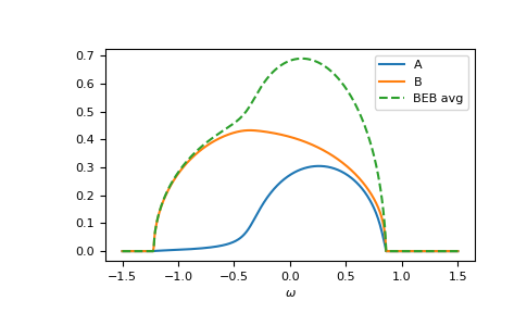
The relevant case is when hopping differs from the CPA case. Then the components can have different band-widths and also the hopping between different components can be different. Let’s say we have two components ‘A’ and ‘B’. The values hopping=np.array([[1.0, 0.5], [0.5, 1.2]]) mean that the hopping amplitude between ‘B’ sites is 1.2 times the hopping amplitude between ‘A’ sites; the hopping amplitude from ‘A’ to ‘B’ is 0.5 times the hopping amplitude between ‘A’ sites.

>>> from functools import partial
>>> e_onsite = np.array([0.2, -0.2])
>>> concentration = np.array([0.3, 0.7])
>>> hopping = np.array([[1.0, 0.5],
...                     [0.5, 1.2]])
>>> g0 = partial(gt.bethe_gf_z, half_bandwidth=1)
>>> ww = np.linspace(-1.5, 1.5, num=501) + 1e-5j

>>> self_beb_ww = gt.beb.solve_root(ww, e_onsite, concentration=concentration,
...                                 hopping=hopping, hilbert_trafo=g0)
>>> gf_loc_ww = gt.beb.gf_loc_z(ww, self_beb_ww, hopping=hopping, hilbert_trafo=g0)
>>> __ = plt.plot(ww.real, -1/np.pi*gf_loc_ww[..., 0].imag, label="A")
>>> __ = plt.plot(ww.real, -1/np.pi*gf_loc_ww[..., 1].imag, label="B")
>>> __ = plt.plot(ww.real, -1/np.pi*gf_loc_ww.sum(axis=-1).imag,
...              linestyle='--', label="BEB avg")
>>> __ = plt.legend()
>>> __ = plt.xlabel(r"$\omega$")
>>> plt.show()

(png, pdf)

Additional diagnostic output is logged, you can get information on the convergence by setting:

>>> import logging
>>> logging.basicConfig()
>>> logging.getLogger('gftool.beb').setLevel(logging.DEBUG)

Matrix Green’s functions via diagonalization

The module gftool.matrix contains some helper functions for matrix diagonalization. A main use case is to calculate the one-particle Green’s function from the resolvent. Instead of inverting the matrix for every frequency point, we can diagonalize the Hamiltonian once:

\[G(z) = [1z - H]^{-1} = [1z - UλU^†]^{-1} = U [z-λ]^{-1} U^†\]

Let’s consider the simple example of a 2D square lattice with nearest-neighbor hopping. The Hamiltonian can be easily constructed:

>>> N = 21   # system size in one dimension
>>> t = tx = ty = 0.5  # hopping amplitude
>>> hamilton = np.zeros([N]*4)
>>> diag = np.arange(N)
>>> hamilton[diag[1:], :, diag[:-1], :] = hamilton[diag[:-1], :, diag[1:], :] = -tx
>>> hamilton[:, diag[1:], :, diag[:-1]] = hamilton[:, diag[:-1], :, diag[1:]] = -ty
>>> ham_mat = hamilton.reshape(N**2, N**2)  # turn in into a matrix

Let’s diagonalize it using the helper in gftool.matrix and calculated the Green’s function

>>> dec = gt.matrix.decompose_her(ham_mat)
>>> ww = np.linspace(-2.5, 2.5, num=201) + 1e-1j  # frequency match
>>> gf_ww = dec.reconstruct(1.0/(ww[:, np.newaxis] - dec.eig))
>>> gf_ww = gf_ww.reshape(ww.size, *[N]*4)  # reshape for easy access

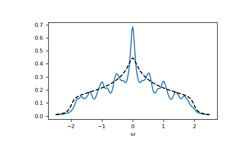
Where we used reconstruct to calculate the matrix product for the given diagonal matrix. Let’s check the local spectral function of the central lattice site:

>>> __ = plt.plot(ww.real, -1.0/np.pi*gf_ww.imag[:, N//2, N//2, N//2, N//2])
>>> __ = plt.plot(ww.real, -1.0/np.pi*gt.square_gf_z(ww, half_bandwidth=4*t).imag,
...               color='black', linestyle='--')
>>> __ = plt.xlabel(r"$\omega$")
>>> plt.show()

(png, pdf)

Oftentimes we are only interested in the local Green’s functions and can avoid a large part of the computation, only calculating the diagonal elements. This can be done using the kind argument:

>>> gf_diag = dec.reconstruct(1.0/(ww[:, np.newaxis] - dec.eig), kind='diag')
>>> gf_diag = gf_diag.reshape(ww.size, N, N)