gftool.fourier.iw2tau

gftool.fourier.iw2tau(gf_iw, beta, moments=(1.0, ), fourier=<function iw2tau_dft>, n_fit=0)

Discrete Fourier transform of the Hermitian Green’s function gf_iw.

Fourier transformation of a fermionic Matsubara Green’s function to imaginary-time domain. We assume a Hermitian Green’s function gf_iw, i.e. \(G(-iω_n) = G^*(iω_n)\), which is the case for commutator Green’s functions \(G_{AB}(τ) = ⟨A(τ)B⟩\) with \(A = B^†\). The Fourier transform gf_tau is then real.

Parameters

gf_iw(…, N_iw) complex np.ndarray

The Green’s function at positive fermionic Matsubara frequencies \(iω_n\).

betafloat

The inverse temperature \(beta = 1/k_B T\).

moments(…, m) float array_like

High-frequency moments of gf_iw.

fourier{iw2tau_dft, iw2tau_dft_soft}, optional

Back-end to perform the actual Fourier transformation.

n_fitint, optional

Number of additionally fitted moments (in fact, gf_iw is fitted, not not directly moments).

Returns

gf_tau(…, 2*N_iw + 1) float np.ndarray

The Fourier transform of gf_iw for imaginary times \(τ \in [0, β]\).

See also

iw2tau_dft

Back-end: plain implementation of Fourier transform

iw2tau_dft_soft

Back-end: Fourier transform with artificial softening of oszillations

pole_gf_from_moments

Function handling the given moments

Notes

For accurate an accurate Fourier transform, it is necessary, that gf_iw has already reached it’s high-frequency behaviour, which need to be included explicitly. Therefore, the accuracy of the FT depends implicitely on the bandwidth!

Examples

>>> BETA = 50
>>> iws = gt.matsubara_frequencies(range(1024), beta=BETA)
>>> tau = np.linspace(0, BETA, num=2*iws.size + 1, endpoint=True)

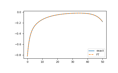
>>> poles = 2*np.random.random(10) - 1  # partially filled
>>> weights = np.random.random(10)
>>> weights = weights/np.sum(weights)
>>> gf_iw = gt.pole_gf_z(iws, poles=poles, weights=weights)
>>> gf_dft = gt.fourier.iw2tau(gf_iw, beta=BETA)
>>> gf_iw.size, gf_dft.size
(1024, 2049)
>>> gf_tau = gt.pole_gf_tau(tau, poles=poles, weights=weights, beta=BETA)

>>> import matplotlib.pyplot as plt
>>> __ = plt.plot(tau, gf_tau, label='exact')
>>> __ = plt.plot(tau, gf_dft, '--', label='FT')
>>> __ = plt.legend()
>>> plt.show()

(png, pdf)

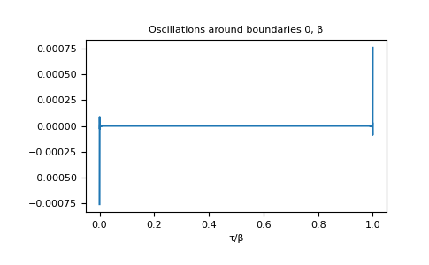
>>> __ = plt.title('Oscillations around boundaries 0, β')
>>> __ = plt.plot(tau/BETA, gf_tau - gf_dft)
>>> __ = plt.xlabel('τ/β')
>>> plt.show()

(png, pdf)

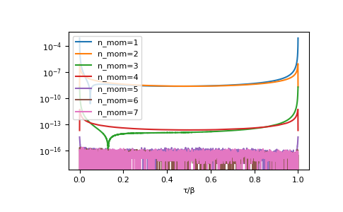
Results can be drastically improved giving high-frequency moments, this reduces the truncation error.

>>> mom = np.sum(weights[:, np.newaxis] * poles[:, np.newaxis]**range(8), axis=0)
>>> for n in range(1, 8):
...     gf = gt.fourier.iw2tau(gf_iw, moments=mom[:n], beta=BETA)
...     __ = plt.plot(tau/BETA, abs(gf_tau - gf), label=f'n_mom={n}')
>>> __ = plt.legend()
>>> __ = plt.xlabel('τ/β')
>>> plt.yscale('log')
>>> plt.show()

(png, pdf)

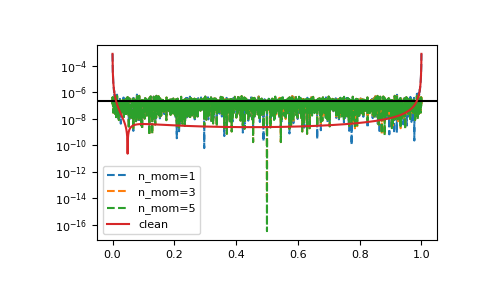
The method is resistant against noise:

>>> magnitude = 2e-7
>>> noise = np.random.normal(scale=magnitude, size=gf_iw.size)
>>> for n in range(1, 7, 2):
...     gf = gt.fourier.iw2tau(gf_iw+noise, moments=mom[:n], beta=BETA)
...     __ = plt.plot(tau/BETA, abs(gf_tau - gf), '--', label=f'n_mom={n}')
>>> __ = plt.axhline(magnitude, color='black')
>>> __ = plt.plot(tau/BETA, abs(gf_tau - gf_dft), label='clean')
>>> __ = plt.legend()
>>> plt.yscale('log')
>>> plt.show()

(png, pdf)