gftool.fourier.izp2tau

gftool.fourier.izp2tau(izp, gf_izp, tau, beta, moments=(1.0))

Fourier transform of the Hermitian Green’s function gf_izp to tau.

Fourier transformation of a fermionic Padé Green’s function to imaginary-time domain. We assume a Hermitian Green’s function gf_izp, i.e. \(G(-iω_n) = G^*(iω_n)\), which is the case for commutator Green’s functions \(G_{AB}(τ) = ⟨A(τ)B⟩\) with \(A = B^†\). The Fourier transform gf_tau is then real.

TODO: this function is not vectorized yet.

Parameters

izp, gf_izp(N_izp) float np.ndarray

Positive fermionic Padé frequencies \(iz_p\) and the Green’s function at specified frequencies.

tau(N_tau) float np.ndarray

Imaginary times 0 <= tau <= beta at which the Fourier transform is evaluated.

betafloat

The inverse temperature \(beta = 1/k_B T\).

moments(m) float array_like, optional

High-frequency moments of gf_izp.

Returns

gf_tau(N_tau) float np.ndarray

The Fourier transform of gf_izp for imaginary times tau.

See also

iw2tau

Fourier transform from fermionic Matsubara frequencies.

_z2polegf

Function handling the fitting of gf_izp

Notes

The algorithm performs in fact an analytic continuation instead of a Fourier integral. It is however only evaluated on the imaginary axis, so far the algorithm was observed to be stable

Examples

>>> BETA = 50
>>> izp, __ = gt.pade_frequencies(50, beta=BETA)
>>> tau = np.linspace(0, BETA, num=2049, endpoint=True)

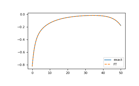
>>> poles = 2*np.random.random(10) - 1  # partially filled
>>> weights = np.random.random(10)
>>> weights = weights/np.sum(weights)
>>> gf_izp = gt.pole_gf_z(izp, poles=poles, weights=weights)
>>> gf_ft = gt.fourier.izp2tau(izp, gf_izp, tau, beta=BETA)
>>> gf_tau = gt.pole_gf_tau(tau, poles=poles, weights=weights, beta=BETA)

>>> import matplotlib.pyplot as plt
>>> __ = plt.plot(tau, gf_tau, label='exact')
>>> __ = plt.plot(tau, gf_ft, '--', label='FT')
>>> __ = plt.legend()
>>> plt.show()

(png, pdf)

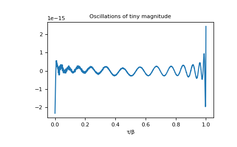
>>> __ = plt.title('Oscillations of tiny magnitude')
>>> __ = plt.plot(tau/BETA, gf_tau - gf_ft)
>>> __ = plt.xlabel('τ/β')
>>> plt.show()

(png, pdf)

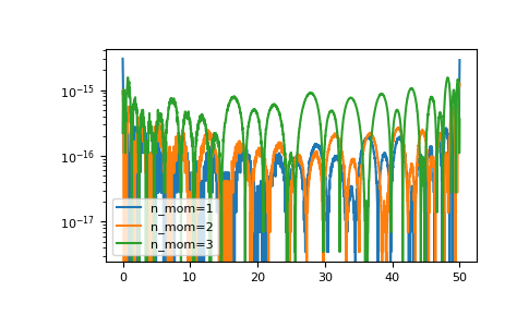
Results of izp2tau can be improved giving high-frequency moments.

>>> mom = np.sum(weights[:, np.newaxis] * poles[:, np.newaxis]**range(4), axis=0)
>>> for n in range(1, 4):
...     gf = gt.fourier.izp2tau(izp, gf_izp, tau, beta=BETA, moments=mom[:n])
...     __ = plt.plot(tau, abs(gf_tau - gf), label=f'n_mom={n}')
>>> __ = plt.legend()
>>> plt.yscale('log')
>>> plt.show()

(png, pdf)

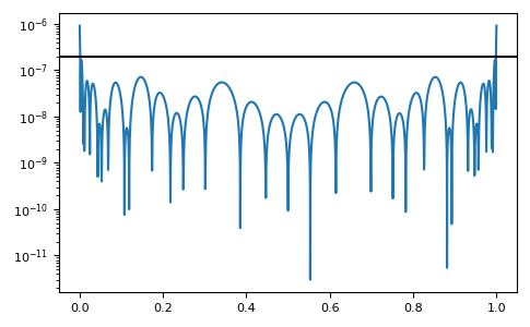
The method is resistant against noise:

>>> magnitude = 2e-7
>>> noise = np.random.normal(scale=magnitude, size=gf_izp.size)
>>> gf = gt.fourier.izp2tau(izp, gf_izp + noise, tau, beta=BETA, moments=(1,))
>>> __ = plt.plot(tau/BETA, abs(gf_tau - gf))
>>> __ = plt.axhline(magnitude, color='black')
>>> plt.yscale('log')
>>> plt.tight_layout()
>>> plt.show()

(png, pdf)

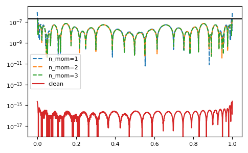
>>> for n in range(1, 4):
...     gf = gt.fourier.izp2tau(izp, gf_izp + noise, tau, beta=BETA, moments=mom[:n])
...     __ = plt.plot(tau/BETA, abs(gf_tau - gf), '--', label=f'n_mom={n}')
>>> __ = plt.axhline(magnitude, color='black')
>>> __ = plt.plot(tau/BETA, abs(gf_tau - gf_ft), label='clean')
>>> __ = plt.legend()
>>> plt.yscale('log')
>>> plt.tight_layout()
>>> plt.show()

(png, pdf)