gftool.lattice.kagome.dos_mp

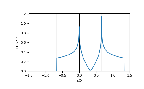
gftool.lattice.kagome.dos_mp(eps, half_bandwidth=1)

Multi-precision DOS of non-interacting 2D kagome lattice.

The delta-peak at eps=-2*half_bandwidth/3 is ommited and must be treated seperately! Without it, the DOS integrates to 2/3.

Besides the delta-peak, the DOS diverges at eps=0 and eps=2*half_bandwidth/3.

Parameters

epsmpmath.mpf or mpf_like

DOS is evaluated at points eps.

half_bandwidthmpmath.mpf or mpf_like

Half-bandwidth of the DOS, DOS(eps < -2/3`half_bandwidth`) = 0, DOS(4/3`half_bandwidth` < eps) = 0. The half_bandwidth corresponds to the nearest neighbor hopping \(t=2D/3\).

Returns

dosfloat np.ndarray or float

The value of the DOS.

See also

gftool.lattice.kagome.dos_mp

vectorized version suitable for array evaluations

gftool.lattice.triangular.dos_mp

gftool.lattice.honeycomb.dos_mp

References

varm2013

Varma, V.K., Monien, H., 2013. Lattice Green’s functions for kagome, diced, and hyperkagome lattices. Phys. Rev. E 87, 032109. https://doi.org/10.1103/PhysRevE.87.032109

kogan2021

Kogan, E., Gumbs, G., 2020. Green’s Functions and DOS for Some 2D Lattices. Graphene 10, 1–12. https://doi.org/10.4236/graphene.2021.101001

Examples

Calculated integrals

>>> from mpmath import mp
>>> mp.identify(mp.quad(gt.lattice.kagome.dos_mp, [-2/3, 0, 1/3, 2/3, 4/3]))
'(2/3)'

>>> eps = np.linspace(-1.5, 1.5, num=1001)
>>> dos_mp = [gt.lattice.kagome.dos(ee, half_bandwidth=1) for ee in eps]

>>> import matplotlib.pyplot as plt
>>> for pos in (-2/3, 0, +2/3):
...     _ = plt.axvline(pos, color='black', linewidth=0.8)
>>> _ = plt.plot(eps, dos_mp)
>>> _ = plt.xlabel(r"$\epsilon/D$")
>>> _ = plt.ylabel(r"DOS * $D$")
>>> _ = plt.ylim(bottom=0)
>>> _ = plt.xlim(left=eps.min(), right=eps.max())
>>> plt.show()

(png, pdf)