gftool.cpa.solve_fxdocc_root

gftool.cpa.solve_fxdocc_root(iws, e_onsite, concentration, hilbert_trafo: Callable[[complex], complex], beta: float, occ: Optional[float] = None, self_cpa_iw0=None, mu0: float = 0, weights=1, n_fit=0, restricted=True, **root_kwds) → gftool.cpa.RootFxdocc

Determine the CPA self-energy by solving the root problem for fixed occ.

Parameters

iws(N_iw) complex array_like

Positive fermionic Matsubara frequencies.

e_onsite(N_cmpt) float or (…, N_iw, N_cmpt) complex np.ndarray

On-site energy of the components. This can also include a local frequency dependent self-energy of the component sites. If multiple non-frequency dependent on-site energies should be considered simultaneously, pass an on-site energy with N_z=1: e_onsite[…, np.newaxis, :].

concentration(…, N_cmpt) float array_like

Concentration of the different components used for the average.

hilbert_trafoCallable[[complex], complex]

Hilbert transformation of the lattice to calculate the coherent Green’s function.

betafloat

Inverse temperature.

occfloat

Total occupation.

self_cpa_iw0, mu0(…, N_iw) complex np.ndarray and float, optional

Starting guess for CPA self-energy and chemical potential. self_cpa_iw0 implicitly contains the chemical potential mu0, thus they should match.

Returns

root.self_cpa(…, N_iw) complex np.ndarray

The CPA self-energy as the root of self_root_eq.

root.mufloat

Chemical potential for the given occupation occ.

Other Parameters

weights(N_iw) float np.ndarray, optional

Passed to gftool.density_iw. Residues of the frequencies with respect to the residues of the Matsubara frequencies 1/beta. (default: 1.) For Padé frequencies this needs to be provided.

n_fitint, optional

Passed to gftool.density_iw. Number of additionally fitted moments. If Padé frequencies are used, this is typically not necessary. (default: 0)

restrictedbool, optional

Whether self_cpa_z is restricted to self_cpa_z.imag <= 0. (default: True) Note, that even if restricted=True, the imaginary part can get negative within tolerance. This should be removed by hand if necessary.

root_kwds

Additional arguments passed to scipy.optimize.root. method can be used to choose a solver. options=dict(fatol=tol) can be specified to set the desired tolerance tol.

Raises

RuntimeError

If unable to find a solution.

See also

solve_root

Examples

>>> from functools import partial
>>> beta = 30
>>> e_onsite = [-0.3, 0.3]
>>> conc = [0.3, 0.7]
>>> hilbert = partial(gt.bethe_gf_z, half_bandwidth=1)
>>> occ = 0.5,

>>> iws = gt.matsubara_frequencies(range(1024), beta=30)
>>> self_cpa_iw, mu = gt.cpa.solve_fxdocc_root(iws, e_onsite, conc,
...                                            hilbert, occ=occ, beta=beta)

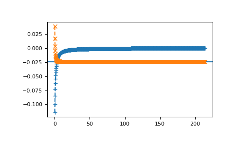
>>> import matplotlib.pyplot as plt
>>> __ = plt.plot(iws.imag, self_cpa_iw.imag, '+--')
>>> __ = plt.axhline(np.average(e_onsite, weights=conc) - mu)
>>> __ = plt.plot(iws.imag, self_cpa_iw.real, 'x--')
>>> plt.show()

(png, pdf)

check occupation

>>> gf_coher_iw = hilbert(iws - self_cpa_iw)
>>> gt.density_iw(iws, gf_coher_iw, beta=beta, moments=[1, self_cpa_iw[-1].real])
0.499999...

check CPA

>>> self_compare = gt.cpa.solve_root(iws, np.array(e_onsite)-mu, conc,
...                                  hilbert_trafo=hilbert)
>>> np.allclose(self_cpa_iw, self_compare, atol=1e-5)
True